
 Tweet
Tweet
As we all (should) know, a single on-axis measurement doesn't really characterize how a speaker sounds. You really have to listen to the speaker.
As I design / observe more speakers with spinorama data, which incorporate measurements in the horizontal plane and vertical plane in 360 degrees:

and presented in this manner:

...it started to dawn on me that although it answers some questions, it leaves out other things. You still have to listen to the speaker.
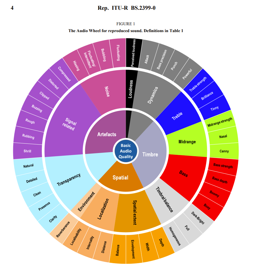
To quote the author/designer of the VituixCAD, things like "non-linear distortion, dynamics, stability of sound balance, timing, level of directivity, diffraction, location of radiators, half space and corner concepts are ignored..."
Reference:
https://kimmosaunisto.net/Software/V...ference_rating
Some of these are unexplored, or at least unpublished in the public domain. Here's what Sean Olive wrote iabout the research that was conducted some 20 years ago:

Reference:
Author's own post on distortion:

I started my own study into non-linear distortion in 2022, but in 2023 I also started a small study on directivity.
To this aim, I've been collecting measurements of high frequency devices. This includes dome tweeters, soft and hard, ribbon tweeters, compression drivers, with and without waveguides or horns, with and without baffles. The goal is to see if measurements can determine the stability of the tonal balance as one moves around the listening area. Or perhaps how it may relate to spatial characteristics, broadly imaging, as one listens from the main listening position. How can measurements help tell us things like:

Reference:
https://extranet.itu.int/brdocsearch...2017-PDF-E.pdf
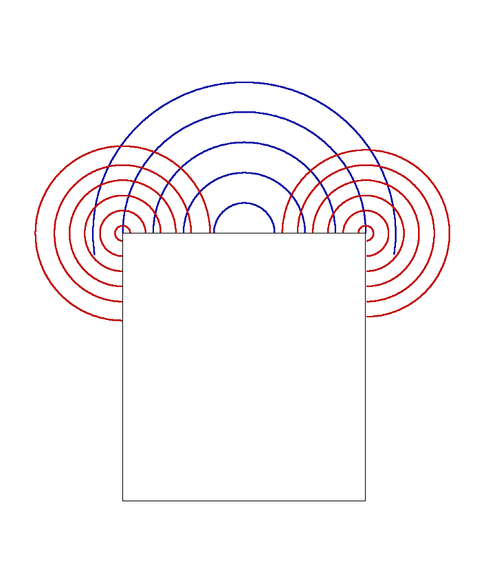
To help with some definitions, I will start off with a theoretical 3/4" tweeter. The graph below represents a circular driver, with a flat diaphragm of 3/4" diameter, flush mounted on a slim 5 1/8" wide x 12" H cabinet. The unit is centered on the baffle, with large 1.5" round-overs.
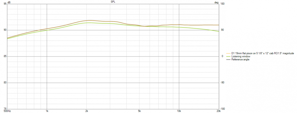
Grey- Reference: On axis response- directly in front of the tweeter, at 1 meter.
Green- Listening window: The average of the on axis, horizontal ±10, horizontal ±20, horizontal ±30, vertical ± 10 responses.
Here is the Directivity chart.
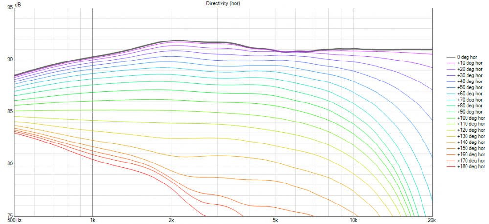
In the past it's has been called dispersion.
lower directivity ~ wider dispersion, and higher directivity ~ narrower dispersion.
constant directivity ~ constant dispersion - as one moves from directly in front to the sides; the sound levels drops evenly for all frequencies.
controlled directivity ~ controlled dispersion - by manipulating how much sound is radiated forwards, sideways, or backwards, we seek to "control the direction" of the sound.
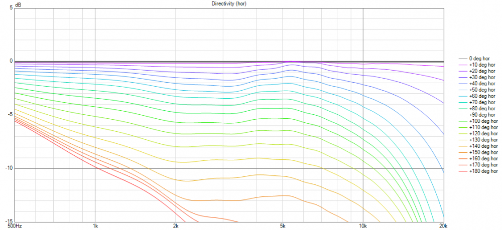
This panel can be converted to normalized line chart, which shows how the frequency responses would behave at off axis angles, when compared to the normal (on-axis) response. Each colored line represents a frequency response measured in angular steps of 10 degrees.
You can also view this as:
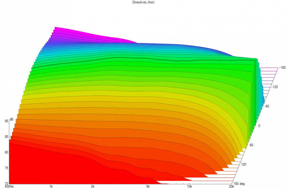
A waterfall chart:
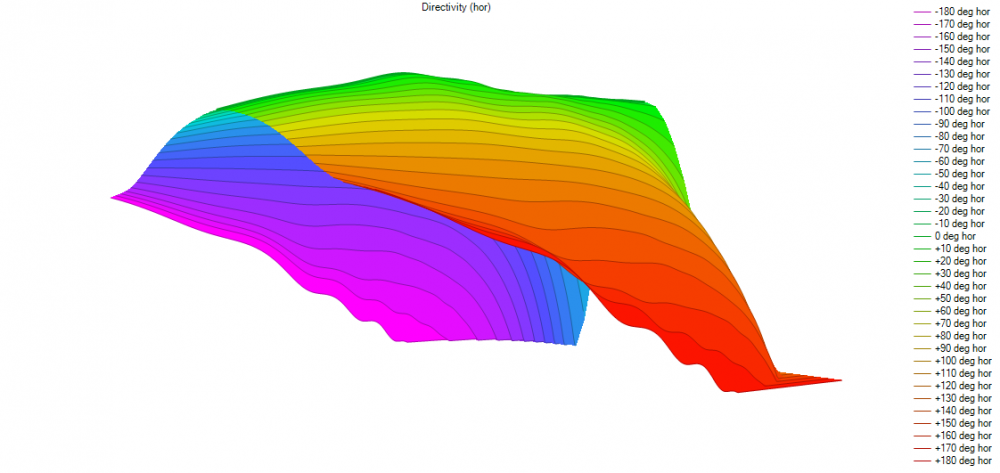
Or a surface chart:
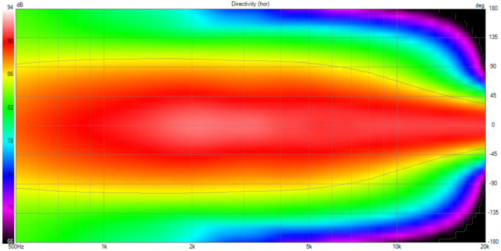
Or a polar map:
Some critics will say that these are all representations of the same data, and they would be correct.
But as I will show, different graphs may be more useful than others to view/understand different things.
For instance, after you’ve seen a few of these big red stripes, you will start to be able to determine beamwidth.
And you will see that it's constant directivity from 500Hz to 5KHz, as it starts to become slightly narrower from 5-20 KHz, it starts to become more directive (higher directivity)
Next up is the Power (response) and Directivity Index chart:
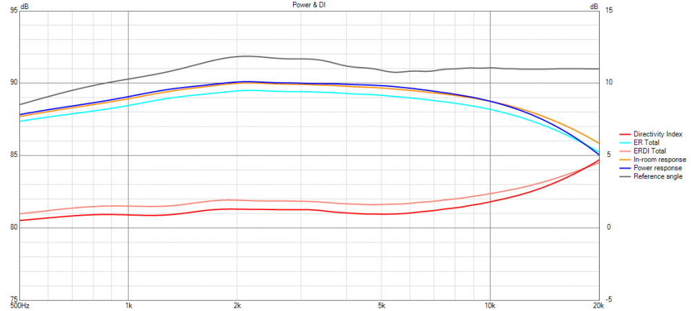
Sound Power Directivity Index (DI) For the purposes of this standard the Sound Power Directivity Index is defined as the difference between the listening window curve and the sound power curve. An SPDI of 0 dB indicates omnidirectional radiation. The larger the SPDI, the more directional the loudspeaker is in the direction of the reference axis
Early Reflections (ER)The early reflections curve is an estimate of all single-bounce, first-reflections, in a typical listening room. • Floor Bounce: 20º, 30º, 40º down • Ceiling Bounce: 40º, 50º, 60º up • Front Wall Bounce: 0º, ± 10º, ± 20º, ± 30º horizontal • Side Wall Bounces: ± 40º, ± 50º, ± 60º, ± 70º, ± 80º horizontal • Rear Wall Bounces: 180º, ± 90º horizonta
Early Reflections Directivity Index (ERDI Total) The Early Reflections Directivity Index is defined as the difference between the listening window curve and the early reflections curve.
(Estimated) In-room response ... a Predicted In-Room (PIR) amplitude response is obtained by a weighted average consisting of 12 % listening window, 44 % early reflections and 44 % sound power.
Power Response: The (sound) power response is the weighted rms average of all 70 measurements, with individual measurements weighted according to the portion of the spherical surface that they represent. Calculation of the sound power curve begins with a conversion from SPL to pressure, a scalar magnitude. The individual measures of sound pressure are then weighted according to the values shown in Appendix C and an energy average (rms) is calculated using the weighted values. The final average is converted to SPL
Reference:
These definitions are covered in:
https://shop.cta.tech/products/standard-method-of-measurement-for-in-home-loudspeaker
As I design / observe more speakers with spinorama data, which incorporate measurements in the horizontal plane and vertical plane in 360 degrees:
and presented in this manner:
...it started to dawn on me that although it answers some questions, it leaves out other things. You still have to listen to the speaker.
To quote the author/designer of the VituixCAD, things like "non-linear distortion, dynamics, stability of sound balance, timing, level of directivity, diffraction, location of radiators, half space and corner concepts are ignored..."
Reference:
https://kimmosaunisto.net/Software/V...ference_rating
Some of these are unexplored, or at least unpublished in the public domain. Here's what Sean Olive wrote iabout the research that was conducted some 20 years ago:
Reference:
Author's own post on distortion:
I started my own study into non-linear distortion in 2022, but in 2023 I also started a small study on directivity.
To this aim, I've been collecting measurements of high frequency devices. This includes dome tweeters, soft and hard, ribbon tweeters, compression drivers, with and without waveguides or horns, with and without baffles. The goal is to see if measurements can determine the stability of the tonal balance as one moves around the listening area. Or perhaps how it may relate to spatial characteristics, broadly imaging, as one listens from the main listening position. How can measurements help tell us things like:
Reference:
https://extranet.itu.int/brdocsearch...2017-PDF-E.pdf
To help with some definitions, I will start off with a theoretical 3/4" tweeter. The graph below represents a circular driver, with a flat diaphragm of 3/4" diameter, flush mounted on a slim 5 1/8" wide x 12" H cabinet. The unit is centered on the baffle, with large 1.5" round-overs.
Grey- Reference: On axis response- directly in front of the tweeter, at 1 meter.
Green- Listening window: The average of the on axis, horizontal ±10, horizontal ±20, horizontal ±30, vertical ± 10 responses.
Here is the Directivity chart.
In the past it's has been called dispersion.
lower directivity ~ wider dispersion, and higher directivity ~ narrower dispersion.
constant directivity ~ constant dispersion - as one moves from directly in front to the sides; the sound levels drops evenly for all frequencies.
controlled directivity ~ controlled dispersion - by manipulating how much sound is radiated forwards, sideways, or backwards, we seek to "control the direction" of the sound.
This panel can be converted to normalized line chart, which shows how the frequency responses would behave at off axis angles, when compared to the normal (on-axis) response. Each colored line represents a frequency response measured in angular steps of 10 degrees.
You can also view this as:
A waterfall chart:
Or a surface chart:
Or a polar map:
Some critics will say that these are all representations of the same data, and they would be correct.
But as I will show, different graphs may be more useful than others to view/understand different things.
For instance, after you’ve seen a few of these big red stripes, you will start to be able to determine beamwidth.
And you will see that it's constant directivity from 500Hz to 5KHz, as it starts to become slightly narrower from 5-20 KHz, it starts to become more directive (higher directivity)
Next up is the Power (response) and Directivity Index chart:
Sound Power Directivity Index (DI) For the purposes of this standard the Sound Power Directivity Index is defined as the difference between the listening window curve and the sound power curve. An SPDI of 0 dB indicates omnidirectional radiation. The larger the SPDI, the more directional the loudspeaker is in the direction of the reference axis
Early Reflections (ER)The early reflections curve is an estimate of all single-bounce, first-reflections, in a typical listening room. • Floor Bounce: 20º, 30º, 40º down • Ceiling Bounce: 40º, 50º, 60º up • Front Wall Bounce: 0º, ± 10º, ± 20º, ± 30º horizontal • Side Wall Bounces: ± 40º, ± 50º, ± 60º, ± 70º, ± 80º horizontal • Rear Wall Bounces: 180º, ± 90º horizonta
Early Reflections Directivity Index (ERDI Total) The Early Reflections Directivity Index is defined as the difference between the listening window curve and the early reflections curve.
(Estimated) In-room response ... a Predicted In-Room (PIR) amplitude response is obtained by a weighted average consisting of 12 % listening window, 44 % early reflections and 44 % sound power.
Power Response: The (sound) power response is the weighted rms average of all 70 measurements, with individual measurements weighted according to the portion of the spherical surface that they represent. Calculation of the sound power curve begins with a conversion from SPL to pressure, a scalar magnitude. The individual measures of sound pressure are then weighted according to the values shown in Appendix C and an energy average (rms) is calculated using the weighted values. The final average is converted to SPL
Reference:
These definitions are covered in:
https://shop.cta.tech/products/standard-method-of-measurement-for-in-home-loudspeaker


Comment